The Phoenix Bird - Swing Trading Strategy - Backtested!

"""
Strategy : Phoenix
Psychology : Sometimes stocks go down in price due to market over-reaction and recovers fast.
This strategy identifies such stocks that hit bottom but is showing signs of recovery.

Rules of strategy:
- This uses daily candles and is run at the end of day to identify potential entries for next day open.
- This is a long-only strategy and hence no shorts
- Strategy will be run after the market is closed for the day and the entry into stock is done the next day open if its satisfies the following conditions.
1. The Rate of change (which is the percentage difference in prices between today's close and close 14 days earlier) is less than -20
2. The Rate of change today is more positive than the rate of change the previous day
3. The Rate of change today is more positive than the rate of change 3 days earlier
- The Target is 1 times ATR range value. The ATR value is to be calculated at the time of entry and maintained at that level till the end of trade
- Stop loss is 2.5 times ATR range value as calculated at the time of entry
- The trade automatically closes if the trade is open for more than 10 days and both target and stoploss are not hit

Custom Modifications:
- Timelimit exit reduced to 10 days (from 20 days)
- Too few trades for -20 ROC limit. Changed it to -15.

"""

import pandas as pd
import numpy as np
import matplotlib.pyplot as plt
from datetime import date
import seaborn as sns


class PhoenixStrategy:
    def __init__(self, tickers, start_date, end_date):
        self.tickers = tickers
        self.ticker = None
        self.start_date = start_date
        self.end_date = end_date
        self.data = None
        self.trades = []
        self.trade_stats = {}

    def fetch_data(self):
        #  Replace this function below with your own function that fetches historic data from your respective broker/resource
        self.data = Instruments.get_historical_data(self.ticker, self.start_date, self.end_date)
        # print(f"Downloaded {len(self.data)} rows of data for {self.ticker}")
        return self.data

    def prepare_data(self):
        # Calculate Rate of Change (ROC) for 14 days
        self.data['ROC_14'] = self.data['Close'].pct_change(14) * 100

        # Calculate ROC from 1 day ago and 3 days ago
        self.data['ROC_14_prev'] = self.data['ROC_14'].shift(1)
        self.data['ROC_14_prev3'] = self.data['ROC_14'].shift(3)

        # Calculate ATR (Average True Range) for setting targets and stop losses
        self.data['TR'] = np.maximum(
            self.data['High'] - self.data['Low'],
            np.maximum(
                abs(self.data['High'] - self.data['Close'].shift(1)),
                abs(self.data['Low'] - self.data['Close'].shift(1))
            )
        )
        self.data['ATR_14'] = self.data['TR'].rolling(window=14).mean()

        # Drop NaN values
        self.data = self.data.dropna()
        return self.data

    def backtest(self):
        # Initialize variables
        in_position = False
        entry_price = 0
        entry_date = None
        entry_atr = 0
        target = 0
        stop_loss = 0
        days_in_trade = 0

        for ticker in self.tickers:
            self.ticker = ticker
            self.fetch_data()
            self.prepare_data()

            # Loop through each day
            for i in range(1, len(self.data)):
                if i == len(self.data)-1:
                    break  # End of data. Avoid error while calculating next_date
                current_date = self.data.index[i]
                prev_date = self.data.index[i - 1]
                next_date = self.data.index[i + 1]

                # If we're in a position, check if any exit conditions are met
                if in_position:
                    days_in_trade += 1
                    high_price = self.data.loc[current_date, 'High']
                    low_price = self.data.loc[current_date, 'Low']
                    close_price = self.data.loc[current_date, 'Close']

                    # Check if target hit during the day
                    if high_price >= target:
                        self.record_trade(entry_date, current_date, entry_price, target, 'target', days_in_trade, entry_atr)
                        print("Target Hit", current_date)
                        in_position = False
                        days_in_trade = 0

                    # Check if stop loss hit during the day
                    elif low_price <= stop_loss:
                        self.record_trade(entry_date, current_date, entry_price, stop_loss, 'stop_loss', days_in_trade,
                                          entry_atr)
                        print("SL Hit", current_date)
                        in_position = False
                        days_in_trade = 0

                    # Check if 10-day limit reached
                    elif days_in_trade >= 10:
                        self.record_trade(entry_date, current_date, entry_price, close_price, 'time_limit', days_in_trade,
                                          entry_atr)
                        print("Time Limit Hit", current_date)
                        in_position = False
                        days_in_trade = 0

                # If not in position, check entry conditions for next day
                else:
                    # Check entry conditions
                    roc_14 = self.data.loc[prev_date, 'ROC_14']
                    roc_14_prev = self.data.loc[prev_date, 'ROC_14_prev']
                    roc_14_prev3 = self.data.loc[prev_date, 'ROC_14_prev3']

                    entry_condition = (
                            # roc_14 < -20 and  # ROC is less than -20%
                            roc_14_prev < -15 and  # ROC is less than -15%
                            roc_14 > roc_14_prev   # ROC today > ROC yesterday
                            and roc_14 > roc_14_prev3  # ROC today > ROC 3 days ago
                    )

                    if entry_condition:
                        # Enter position at next day's open
                        entry_price = self.data.loc[next_date, 'Open']
                        entry_date = next_date

                        entry_atr = self.data.loc[current_date, 'ATR_14']  # Use ATR from previous day (at time of decision)

                        # Set target and stop loss
                        target = entry_price + (entry_atr * 1.0)
                        stop_loss = entry_price - (entry_atr * 2.5)
                        print("Entry Triggered for ", self.ticker," Date ", entry_date, " Price ", entry_price, " Target ", target, " Stop Loss ", stop_loss)
                        in_position = True
                        days_in_trade = 1

        return self.trades

    def record_trade(self, entry_date, exit_date, entry_price, exit_price, exit_reason, days_held, atr):
        pnl = ((exit_price / entry_price) - 1) * 100  # Percentage gain/loss
        pnl_r = pnl / (atr / entry_price * 100)  # R multiple (profit in terms of ATR)

        trade = {
            'entry_date': entry_date,
            'exit_date': exit_date,
            'entry_price': entry_price,
            'exit_price': exit_price,
            'exit_reason': exit_reason,
            'days_held': days_held,
            'pnl_percent': pnl,
            'atr_at_entry': atr,
            'pnl_r': pnl_r
        }

        self.trades.append(trade)
        return trade

    def analyze_performance(self):
        if not self.trades:
            print("No trades were executed in the backtest period.")
            return {}

        # Convert trades to DataFrame for analysis
        trades_df = pd.DataFrame(self.trades)

        # Overall statistics
        total_trades = len(trades_df)
        winning_trades = len(trades_df[trades_df['pnl_percent'] > 0])
        losing_trades = len(trades_df[trades_df['pnl_percent'] <= 0])

        win_rate = winning_trades / total_trades if total_trades > 0 else 0

        avg_win = trades_df[trades_df['pnl_percent'] > 0]['pnl_percent'].mean() if winning_trades > 0 else 0
        avg_loss = trades_df[trades_df['pnl_percent'] <= 0]['pnl_percent'].mean() if losing_trades > 0 else 0

        profit_factor = abs(trades_df[trades_df['pnl_percent'] > 0]['pnl_percent'].sum() /
                            trades_df[trades_df['pnl_percent'] <= 0][
                                'pnl_percent'].sum()) if losing_trades > 0 else float('inf')

        # Total return calculation
        initial_capital = 100000  # Assuming $10,000 starting capital
        capital = initial_capital
        equity_curve = [initial_capital]

        for _, trade in trades_df.iterrows():
            trade_return = trade['pnl_percent'] / 100  # Convert percentage to decimal
            capital = capital * (1 + trade_return)
            equity_curve.append(capital)

        total_return_pct = ((capital - initial_capital) / initial_capital) * 100

        # Calculate drawdown
        peaks = pd.Series(equity_curve).cummax()
        drawdowns = (pd.Series(equity_curve) / peaks - 1) * 100
        max_drawdown = drawdowns.min()

        # Calculate Sharpe Ratio (assuming 252 trading days in a year)
        trade_returns = trades_df['pnl_percent'] / 100
        sharpe_ratio = np.sqrt(total_trades) * trade_returns.mean() / trade_returns.std() if len(
            trade_returns) > 1 else 0

        # Group trades by exit reason
        exit_reasons = trades_df.groupby('exit_reason').agg({
            'pnl_percent': ['count', 'mean', 'sum']
        })

        # Average trade duration
        avg_days_held = trades_df['days_held'].mean()

        # R-multiple statistics
        avg_r = trades_df['pnl_r'].mean()

        # Store all stats in a dictionary
        self.trade_stats = {
            'total_trades': total_trades,
            'winning_trades': winning_trades,
            'losing_trades': losing_trades,
            'win_rate': win_rate,
            'avg_win_pct': avg_win,
            'avg_loss_pct': avg_loss,
            'profit_factor': profit_factor,
            'total_return_pct': total_return_pct,
            'max_drawdown_pct': max_drawdown,
            'sharpe_ratio': sharpe_ratio,
            'avg_trade_duration': avg_days_held,
            'avg_r_multiple': avg_r,
            'exit_reasons': exit_reasons,
            'equity_curve': equity_curve
        }

        return self.trade_stats

    def display_results(self):
        if not self.trade_stats:
            print("No analysis available. Run analyze_performance() first.")
            return

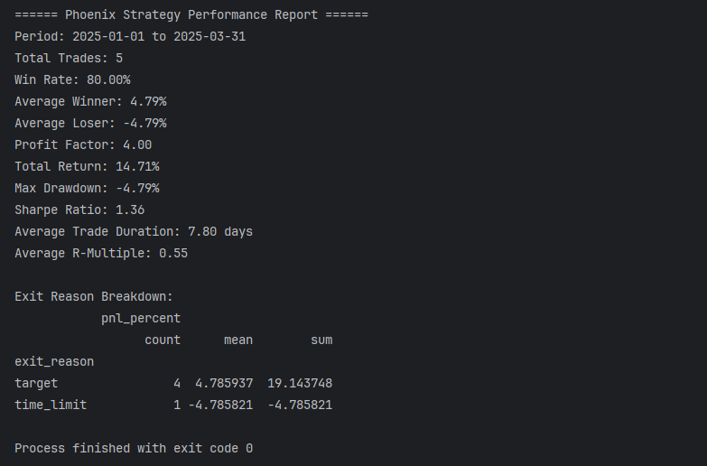
        print("\n====== Phoenix Strategy Performance Report ======")
        # print(f"Symbol: {self.ticker}")
        print(f"Period: {self.start_date} to {self.end_date}")
        print(f"Total Trades: {self.trade_stats['total_trades']}")
        print(f"Win Rate: {self.trade_stats['win_rate']:.2%}")
        print(f"Average Winner: {self.trade_stats['avg_win_pct']:.2f}%")
        print(f"Average Loser: {self.trade_stats['avg_loss_pct']:.2f}%")
        print(f"Profit Factor: {self.trade_stats['profit_factor']:.2f}")
        print(f"Total Return: {self.trade_stats['total_return_pct']:.2f}%")
        print(f"Max Drawdown: {self.trade_stats['max_drawdown_pct']:.2f}%")
        print(f"Sharpe Ratio: {self.trade_stats['sharpe_ratio']:.2f}")
        print(f"Average Trade Duration: {self.trade_stats['avg_trade_duration']:.2f} days")
        print(f"Average R-Multiple: {self.trade_stats['avg_r_multiple']:.2f}")

        # Display exit reason statistics
        print("\nExit Reason Breakdown:")
        print(self.trade_stats['exit_reasons'])

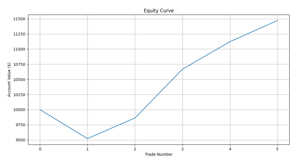
        # Plot equity curve
        plt.figure(figsize=(12, 6))
        plt.plot(self.trade_stats['equity_curve'])
        plt.title('Equity Curve')
        plt.xlabel('Trade Number')
        plt.ylabel('Account Value ($)')
        plt.grid(True)
        plt.show()

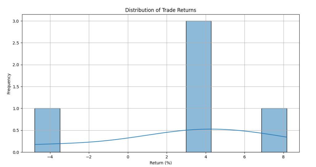
        # Plot distribution of returns
        plt.figure(figsize=(12, 6))
        trades_df = pd.DataFrame(self.trades)
        sns.histplot(trades_df['pnl_percent'], kde=True)
        plt.title('Distribution of Trade Returns')
        plt.xlabel('Return (%)')
        plt.ylabel('Frequency')
        plt.grid(True)
        plt.show()

        # Plot monthly returns
        trades_df['month'] = pd.to_datetime(trades_df['entry_date']).dt.to_period('M')
        monthly_returns = trades_df.groupby('month')['pnl_percent'].sum()

        plt.figure(figsize=(12, 6))
        monthly_returns.plot(kind='bar')
        plt.title('Monthly Returns')
        plt.xlabel('Month')
        plt.ylabel('Return (%)')
        plt.grid(True)
        plt.xticks(rotation=45)
        plt.tight_layout()
        plt.show()

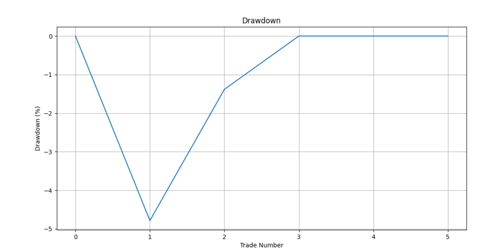
        # Plot drawdown
        equity_series = pd.Series(self.trade_stats['equity_curve'])
        peaks = equity_series.cummax()
        drawdowns = (equity_series / peaks - 1) * 100

        plt.figure(figsize=(12, 6))
        drawdowns.plot()
        plt.title('Drawdown')
        plt.xlabel('Trade Number')
        plt.ylabel('Drawdown (%)')
        plt.grid(True)
        plt.show()

    def run_full_backtest(self):
        self.backtest()
        self.analyze_performance()
        self.display_results()
        return self.trades, self.trade_stats


if __name__ == "__main__":
    pd.set_option("display.max_rows", None, "display.max_columns", None)
    tickers = [
        "INFY", "ITC", "ASIANPAINT", "BRITANNIA", "ICICIBANK", "HCLTECH", "TCS", "LTIM", "TITAN",
        "DRREDDY", "HINDUNILVR", "SBIN", "TATACONSUM", "HDFCBANK", "KOTAKBANK", "MARUTI", "BAJAJFINSV",
        "SBILIFE", "LT", "NESTLEIND","AXISBANK", "CIPLA", "BHARTIARTL", "HEROMOTOCO", "GRASIM", "DIVISLAB",
        "ADANIPORTS","TECHM","SUNPHARMA","EICHERMOT","INDUSINDBK","RELIANCE", "HDFCLIFE", "APOLLOHOSP",
        "M&M","SHRIRAMFIN", "BAJFINANCE","POWERGRID", "ADANIENT", "BAJAJ-AUTO","WIPRO","ULTRACEMCO", "TATAMOTORS",
        "NTPC", "COALINDIA", "ONGC", "HINDALCO", "BPCL", "JSWSTEEL", "TATASTEEL"
    ]

    # Back Test period
    start_date = date(2025, 1, 1)  # Modify as needed
    end_date = date(2025, 3, 31)  # Modify as needed

    strategy = PhoenixStrategy(tickers, start_date, end_date)
    trades, stats = strategy.run_full_backtest()