Investing
Trending + Value Stocks = 96.9% Returns?!

FabTrader
Investors are constantly looking for strategies that maximize returns while minimizing risk. One such strategy that has gained traction is the Trending Value Portfolio, a concept originally proposed by James O'Shaughnessy in his book What Works on Wall Street. This approach combines the best of momentum investing and value investing to identify stocks that are both fundamentally strong and currently trending upward in the market.
Understanding the Two Key Elements
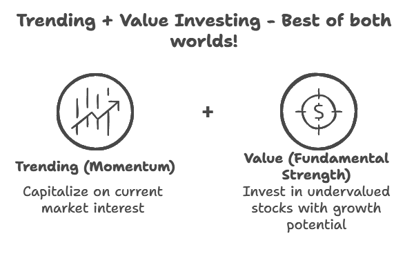
The Trending Value strategy relies on two critical aspects:
Trending (Momentum)
This refers to stocks that have shown strong price momentum over the last six months, attracting significant investor interest.
Stocks are sorted in descending order based on their six-month return performance.
The idea is to invest in stocks that are already gaining traction, ensuring that investors ride the wave of market interest.
Value (Fundamental Strength)
These are stocks that are fundamentally strong but remain undervalued by the market.
The goal is to identify these hidden gems early, allowing investors to capitalize on their future growth potential.
Value investing traditionally focuses on stocks that have strong financials but are trading at a discount to their intrinsic value.
In this article, we will explore the technical workings of the Token method, explain how to implement it in Python, and discuss its advantages and limitations. We will also provide a Python script that automates the login process and demonstrates how to fetch user profile information using the encrypted token.
Why Combine Momentum and Value Investing?
Historically, Momentum Investing and Value Investing were treated as independent strategies. However, O'Shaughnessy demonstrated that a synergy exists when combining them. The results from his backtesting showed:
- Investing in the full S&P 500 yielded an average annual return of 11.2%.
- Investing in the top momentum stocks (six-month highest returns) increased returns to 14.5%.
- Investing in undervalued stocks (based on the Value Composite 2 score) returned 17.3%.
- Trending Value Portfolio, which combines both approaches, delivered the highest return at 21.2%!
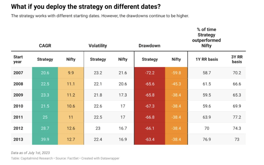
Where's the proof?
Our friends at Capitalminds have done an excellent job of breaking down this strategy and has done extensive back test on this. Refer to their article here
Shankar Nath, the popular youtuber has done his own set of back tests and has claimed that this strategy gave him a 96.9% return! Video
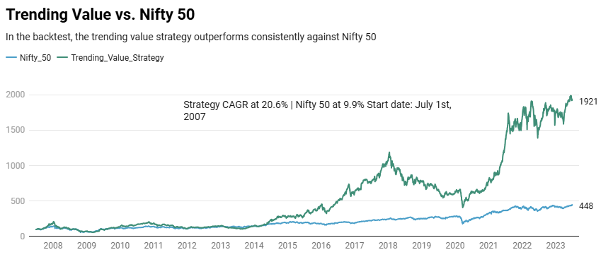
Courtesy : Capitalminds
The Value Composite Score
To identify undervalued stocks, O'Shaughnessy introduced the Value Composite Score, which is calculated using six key financial metrics:
- Price-to-Earnings (P/E) Ratio – Lower is better (indicates undervaluation).
- Price-to-Book (P/B) Ratio – Lower is better (compares market cap to net assets).
- Price-to-Cash Flow (P/CF) Ratio – Lower is better (compares market cap to cash flow from operations).
- Price-to-Sales (P/S) Ratio – Lower is better (compares market cap to revenue).
- EV/EBITDA Ratio – Lower is better (compares enterprise value to earnings before interest, tax, depreciation, and amortization).
- Dividend Yield – Higher is better (indicates a stronger return to shareholders).
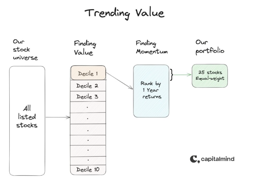
How the Trending Value Portfolio is Constructed
- Assign a decile rank (1 to 10) to each stock for each of the six value parameters.
- Sum up all decile ranks to create a consolidated score.
- Re-rank the consolidated scores and retain only the top 10% (best-ranked decile).
- Sort the shortlisted stocks based on their six-month momentum performance.
- Select the top 25 stocks from the final ranked list to construct the portfolio.
Stock Universe: Where to Look?
The Trending Value Portfolio focuses on stocks with a market capitalization of more than ₹500 crore. This ensures a good mix of small-cap and micro-cap stocks, which tend to offer high growth potential while maintaining reasonable liquidity.
Why 25 Stocks?
Backtesting by O'Shaughnessy showed that a 25-stock portfolio provided the best risk-adjusted returns. A smaller portfolio increases volatility, while a larger one dilutes potential gains.
Rebalancing Strategy
To maintain efficiency, the Trending Value Portfolio must be rebalanced either quarterly or semiannually. The process includes:
- Running the stock screener every three or six months.
- Selling stocks that have dropped out of the top-ranked list.
- Replacing them with new high-ranking stocks that meet the criteria.
Access this Screener for Free
You can access this screener for free on our community toolset page
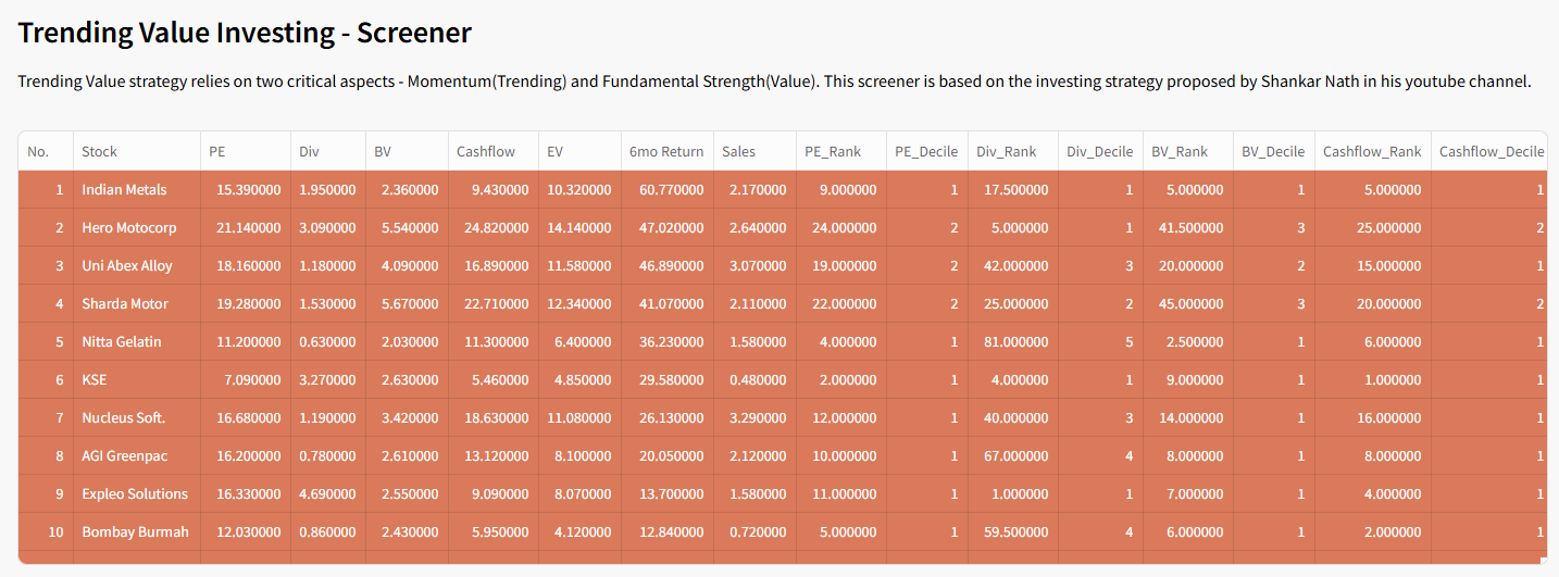
Python Implementation of the automated Screener
I have built this automated python screener that can fetch the 25 stocks per strategy rules with a single click of a button! Try this out and let me know if its useful
"""
Automated Screener for Fetching Trending Value stocks
Reference: Refer to Shankar Nath's Trending Value video for detaile rules
https://www.youtube.com/watch?v=g6xanpDdVNI

-- Dependencies to be installed --
pip install beautifulsoup4==4.11.2
pip install openpyxl
pip install pandas

Disclaimer:
The information provided is for educational and informational purposes only and
should not be construed as financial, investment, or legal advice. The content is based on publicly available
information and personal opinions and may not be suitable for all investors. Investing involves risks,
including the loss of principal.

Author: FabTrader  ([email protected])
www.fabtrader.in
YouTube: @fabtraderinc
X / Instagram / Telegram :  @fabtraderinc
"""

import time
import pandas as pd
import logging

def configure_logging():
    # Configure Application Logging
    log_filepath = "ToolsLog.log"
    format = "%(asctime)s: - %(levelname)s - %(message)s"
    logging.basicConfig(
            filename=log_filepath,
            format=format,
            level=logging.INFO,
            datefmt="%Y-%m-%d %H:%M:%S")

def fetch_screener_data(link):
    cache_index = None
    data = pd.DataFrame()
    current_page = 1
    page_limit = 25
    while current_page < page_limit:

        if current_page == 1:
            url=link
        else:
            url = f'{link}?page={current_page}'

        all_tables = pd.read_html(url, flavor='bs4')
        combined_df = pd.concat(all_tables)

        combined_df = combined_df.drop(
            combined_df[combined_df['S.No.'].isnull()].index)

        # print(combined_df)
        # if cache_index == combined_df.iloc[-2]['S.No.']:
        if len(combined_df.index) < 26:
            data = pd.concat([data, combined_df], axis=0)
            break
        # cache_index = combined_df.iloc[-2]['S.No.']
        # print(cache_index)
        data = pd.concat([data, combined_df], axis=0)
        current_page += 1
        time.sleep(1)
    data = data.iloc[0:].drop(data[data['S.No.'] == 'S.No.'].index)

    return data

pd.set_option("display.max_rows", None, "display.max_columns", None)

configure_logging()

logging.info("Tools : Trending Value Screen extract commenced")
# Fetch PE/PB/Dividend Yield Value Ratio
pbv_link = 'https://www.screener.in/screens/2112737/trendvalue_pricebookvalue/'
pbv_df = fetch_screener_data(pbv_link)
pbv_df = pbv_df[['Name','P/E', 'Div Yld  %', 'CMP / BV']]
pbv_df['P/E'] = pd.to_numeric(pbv_df['P/E'], errors='coerce')
pbv_df['Div Yld  %'] = pd.to_numeric(pbv_df['Div Yld  %'], errors='coerce')
pbv_df['CMP / BV'] = pd.to_numeric(pbv_df['CMP / BV'], errors='coerce')
pbv_df['P/E'] = pbv_df['P/E'].fillna(100000)
pbv_df['CMP / BV'] = pbv_df['CMP / BV'].fillna(100000)
pbv_df['Div Yld  %'] = pbv_df['Div Yld  %'].fillna(0)
# pbv_df.to_excel('D:/pbv.xlsx', index=False)
pbv_df.dropna(inplace=True)
pbv_df = pbv_df[pbv_df['P/E'] > 0]
pbv_df = pbv_df[pbv_df['Div Yld  %'] > 0]
merged_df = pbv_df

# Fetch Price to Free Cash Flow
cashflow_link = 'https://www.screener.in/screens/2112756/trendvalue_cashflow/'
cf_df = fetch_screener_data(cashflow_link)
cf_df = cf_df[['Name','CMP / OCF']]
cf_df['CMP / OCF'] = pd.to_numeric(cf_df['CMP / OCF'], errors='coerce')
cf_df['CMP / OCF'] = cf_df['CMP / OCF'].fillna(100000)
# cf_df.to_excel('D:/cashflow.xlsx', index=False)
cf_df.dropna(inplace=True)
cf_df = cf_df[cf_df['CMP / OCF'] > 0]
merged_df = pd.merge(merged_df, cf_df, on='Name', how='inner')
# print("Free Cash Flow data extraction complete")

# Fetch EV to EBITDA
ev_link = 'https://www.screener.in/screens/2112767/trendvalue_ev/'
ev_df = fetch_screener_data(ev_link)
ev_df = ev_df[['Name','EV / EBITDA']]
ev_df['EV / EBITDA'] = pd.to_numeric(ev_df['EV / EBITDA'], errors='coerce')
ev_df['EV / EBITDA'] = ev_df['EV / EBITDA'].fillna(100000)
# ev_df.to_excel('D:/ev.xlsx', index=False)
ev_df.dropna(inplace=True)
ev_df = ev_df[ev_df['EV / EBITDA'] > 0]
merged_df = pd.merge(merged_df, ev_df, on='Name', how='inner')
# print("EV to EBDITA data extraction complete")

# Fetch Price to Sales ratio
sales_link = 'https://www.screener.in/screens/2112772/trendvalue_pricesales/'
sales_df = fetch_screener_data(sales_link)
sales_df = sales_df[['Name','CMP / Sales']]
sales_df['CMP / Sales'] = pd.to_numeric(sales_df['CMP / Sales'], errors='coerce')
sales_df['CMP / Sales'] = sales_df['CMP / Sales'].fillna(100000)
# sales_df.to_excel('D:/sales.xlsx', index=False)
sales_df.dropna(inplace=True)
sales_df = sales_df[sales_df['CMP / Sales'] > 0]
# print("Price to Sales Ratio data extraction complete")

# Fetch Last 6 months return (Momentum)
momentum_link = 'https://www.screener.in/screens/2112742/trendvalue_momentum/'
mo_df = fetch_screener_data(momentum_link)
mo_df = mo_df[['Name','6mth return  %']]
mo_df['6mth return  %'] = pd.to_numeric(mo_df['6mth return  %'], errors='coerce')
mo_df['6mth return  %'] = mo_df['6mth return  %'].fillna(-100000)
# mo_df.to_excel('D:/mo.xlsx', index=False)
mo_df.dropna(inplace=True)
mo_df = mo_df[mo_df['6mth return  %'] > 0]
merged_df = pd.merge(merged_df, mo_df, on='Name', how='inner')
# print("Momentum / 6 month Returns data extraction complete")

# Final Merged dataset
merged_df = pd.merge(merged_df, sales_df, on='Name', how='inner')
merged_df = merged_df.rename(columns={
    'Name': 'Stock',
    'P/E': 'PE',
    'Div Yld  %': 'Div',
    'CMP / BV': 'BV',
    'CMP / OCF': 'Cashflow',
    'EV / EBITDA': 'EV',
    'CMP / Sales': 'Sales',
    '6mth return  %': '6mo Return'
})
merged_df['PE'] = merged_df['PE'].map(lambda x: float(x))
merged_df['Div'] = merged_df['Div'].map(lambda x: float(x))
merged_df['BV'] = merged_df['BV'].map(lambda x: float(x))
merged_df['6mo Return'] = merged_df['6mo Return'].map(lambda x: float(x))
# merged_df['3mo Return'] = merged_df['3mo Return'].map(lambda x: float(x))
merged_df['Cashflow'] = merged_df['Cashflow'].map(lambda x: float(x))
merged_df['EV'] = merged_df['EV'].map(lambda x: float(x))
merged_df['Sales'] = merged_df['Sales'].map(lambda x: float(x))

# Apply Decile for PE
merged_df['PE_Rank'] = merged_df['PE'].rank()
merged_df['PE_Decile'] = pd.qcut(merged_df['PE_Rank'], q=10, labels=False, duplicates='drop') + 1

# Apply Decile for Div
merged_df['Div_Rank'] = merged_df['Div'].rank(ascending=False)
merged_df['Div_Decile'] = pd.qcut(merged_df['Div_Rank'], q=10, labels=False, duplicates='drop') + 1

# Apply Decile for BV
merged_df['BV_Rank'] = merged_df['BV'].rank()
merged_df['BV_Decile'] = pd.qcut(merged_df['BV_Rank'], q=10, labels=False, duplicates='drop') + 1

# Apply Decile for Cashflow
merged_df['Cashflow_Rank'] = merged_df['Cashflow'].rank()
merged_df['Cashflow_Decile'] = pd.qcut(merged_df['Cashflow_Rank'], q=10, labels=False, duplicates='drop') + 1

# Apply Decile for EV
merged_df['EV_Rank'] = merged_df['EV'].rank()
merged_df['EV_Decile'] = pd.qcut(merged_df['EV_Rank'], q=10, labels=False, duplicates='drop') + 1

# Apply Decile for Sales
merged_df['Sales_Rank'] = merged_df['Sales'].rank()
merged_df['Sales_Decile'] = pd.qcut(merged_df['Sales_Rank'], q=10, labels=False, duplicates='drop') + 1

# Consolidated_Rank column
merged_df['Consolidated_Rank'] = merged_df['PE_Decile'] + merged_df['Div_Decile'] + merged_df['BV_Decile'] + merged_df['Cashflow_Decile'] + merged_df['EV_Decile'] + merged_df['Sales_Decile']

# Retain only stocks that has given a postive return in the last 6 months
merged_df = merged_df[merged_df['6mo Return'] > 0]

# Decile on consolidated rank
merged_df['Consolidated_Decile'] = pd.qcut(merged_df['Consolidated_Rank'], q=10, labels=False, duplicates='drop') + 1
merged_df = merged_df.sort_values(by=['Consolidated_Decile', '6mo Return'], ascending=[True, False])
merged_df.to_excel('data/merged.xlsx', index=False)

# Retain only rows in the first decile of Consolidated_Decile
df_final = merged_df[merged_df['Consolidated_Decile'] == 1]
# df_final = df_final.head(25)
df_final.to_excel('data/final.xlsx', index=False)
print("Final Dataset")
print(df_final)

logging.info("Tools : Trending Value Screen extract completed")
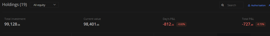
Current Status of the Model Portfolio (as on 31-Aug-2025)
Following is the current status of this portfolio. I have not managed to rebalance this yet. This investment started on the 26th of Sep 2024, which coincidentally was the time Nifty also plunged into a bear phase and has not recovered from that position yet. Nifty is down -7% and this portfolio is down -0.73%.
Conclusion: Why Trending Value Works
The Trending Value Portfolio is a powerful strategy that leverages both market momentum and fundamental strength. By combining the best aspects of momentum investing (trending stocks) and value investing (undervalued stocks), this approach has historically outperformed traditional investment strategies.
For investors looking to enhance their portfolio returns while maintaining a disciplined, systematic approach, Trending Value Investing offers a proven, data-backed method to achieve superior gains.
More from Investing
Beyond Returns: Why I Built a More Intelligent Midcap Mutual Fund Screener
Looking for the best midcap mutual funds in India? This article explains how our Midcap Mutual Fund Screener goes beyond traditional return-based...
How to Build a robust Passive Index Investing System that works
Passive investing has transformed the way investors build wealth. But with so many choices—from Nifty 50 Index Funds and Nifty Next 50...
A Simple, Peaceful ETF Rotation Strategy That Delivered 32% CAGR
Markets are constantly shifting leadership between sectors, asset classes, and global markets. Instead of trying to predict where the next opportunity might...